Data Mining and Knowledge Discovery

1 Association Rule Mining

1.1 Definitions

n-itemset: Number of items in a set. Example: {B,C} is a 2-itemset.

support: Time of an itemset appears in the dataset.

Large item sets: item sets with support ≥ a threshold

Association rule, Support and Confidence

• Rule: X → Y . For example: {B,C} → E
• Support: The support of a rule equals to the support of {X,Y}
• Confidence: $Support(Y)/Support(X)$

We want to find association rules with Support > a threshold & Confidence > a threshold in association rule mining.

K-frequent N-itemset: Item sets whose support is at least K and having N items.

---

1.2 A priori

Two property

1. If an itemset S is large, then any proper subset of S must be large.
2. If an itemset S is NOT large, then any proper superset of S must NOT be large.

Algorithm of A priori Method

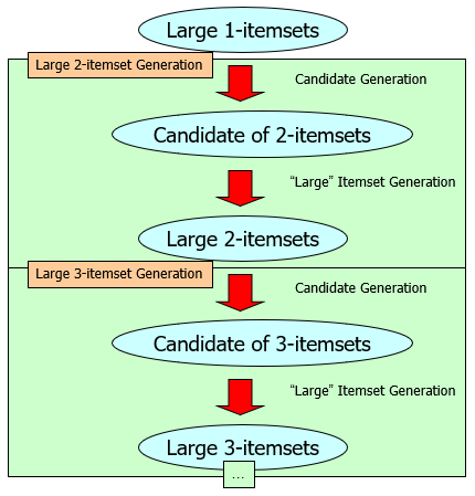
Candidate Generation: Join and Prune

Join Step:

• Input: $L_{k-1}$, a set of large (k-1)-itemsets

• Output: $C_k$, a set of candidates k-itemsets

• Algorithm:

  ​ Select two large k-1 itemsets p and q with the same prefix

  ​ Insert into $C_k$: p and the last item of q, where $q.item_{k-1} > p.item_{k-1}$

Prune Step:

• For all itemsets in $c\in C_{k}$ , do:
  • For all (k-1)-subsets s of c , do:
    • if s not large, delete c form k.

After the candidate generation with Join Step and Prune Step, scan the database to obtain the count of each itemset in the candidate set then produce $L_k$

---

1.3 FP-Tree

Disadvantage of apriori method: 1. It’s costly to handle a large number of candidate sets. 2. It is tedious to repeatedly scan the whole database.

FP-tree only scan the database once to store all essential information in the tree.

FP-tree steps:

1. Deduce the ordered frequent items. For items with the same frequency, the order is given by the alphabetical order.
2. Construct the FP-tree from the above data.
3. From the FP-tree above, construct the FP-conditional tree for each item (or itemset).
4. Determine the frequent patterns.

Example (Threshold=3)

Step1: Deduce the ordered frequent items. For items with the same frequency, the order is given by the alphabetical order.

Step2: Construct the FP-tree from the above data.

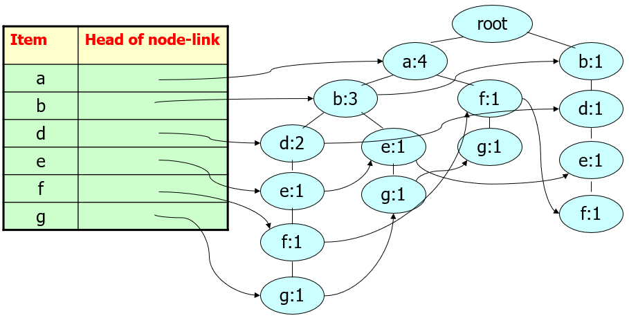
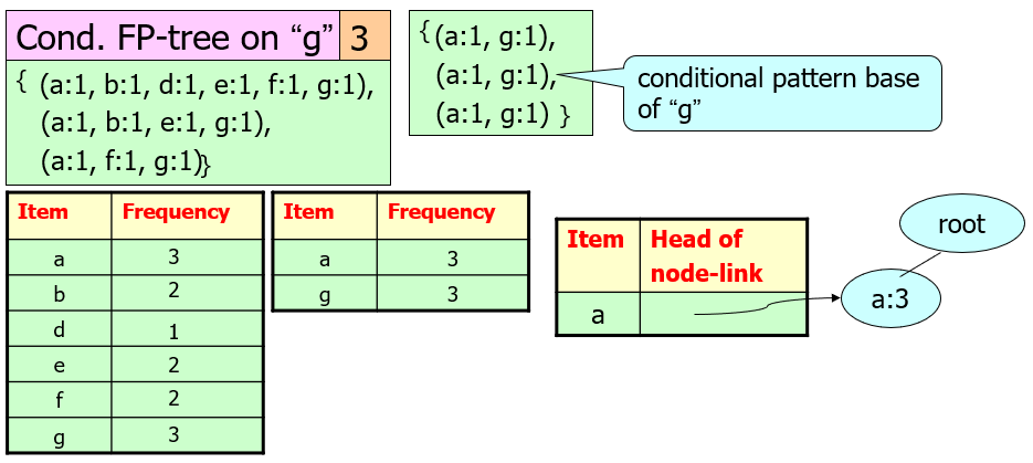
Step3: From the FP-tree above, construct the FP-conditional tree for each item (or itemset).

(From all nodes with “g”, reverse to the root from this node)

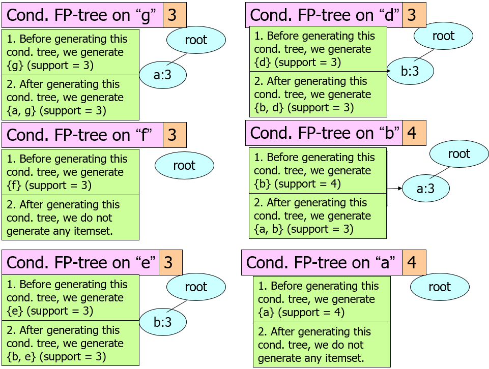
Step4: Determine the frequent patterns.

Complexity of FP-tree:

Require two scans of the transactions DB: Collect Frequent Items and Construct the FP-tree.

Cost to insert one transaction: Number of frequent items in this transaction.

The size of the FP-tree is bounded by the overall occurrences of the frequent items in the database.

The height of the tree is bounded by the maximum number of frequent items in any transaction in the database

---

2 Clustering

2.1 K-means Clustering

Suppose we have n example feature vectors and we know that they fall into k compact clusters.

Let $m_i$ be the mean of the vectors in cluster $i$. We can say that $x$ is in cluster $i$ if distance from $x$ to $m_i$ is the minimum of all the $k$ distances.

Procedure for finding k-means

• Make initial guess for the means: $m_1, m_2, m_3, ..., m_k$

• Until there is no change in any mean:

  • Assign each point to its nearest cluster (mean)
  • Calculate the new mean for each cluster
  • Replace all the means with new means

Initialization of k-means

Randomly choose $k$ of the examples.

The result of K-means clustering depends on the initial means and it frequently happens that suboptimal results are found. The standard solution is to try a number of different initial means.

Disadvantages of k-means

• “Bad” initial guess.
• The value of k is not user-friendly (User cannot choose the best k for unknown data)

2.2 Sequential K-means Clustering

Update the means with one example at a time. Useful when the data is acquired over a period of time.

Procedure for sequential k-means clustering

• Make initial guess for the means: $m_1, m_2, m_3, ..., m_k$
• Set the counts $n_1, n_2, n_3, ..., n_k$ to zero
• Until data is used up / interrupted:
  • Acquire the next example $x$
  • If $m_i$ is closest to $x$
    • Increment $n_i$
    • Replace $m_i$ by $m_i+\frac{1}{n_i}\times(x-m_i)$

2.3 Forgetful Sequential K-means Clustering

Let $a$ be a constant between 0 and 1

Procedure for forgetful sequential k-means clustering

• Make initial guess for the means: $m_1, m_2, m_3, ..., m_k$
• If $m_i$ is closest to $x$, replace $m_i$ by $m_i+a(x-m_i)$

In this method, $m_i$ is a weighted average of the examples that were closest to $m_i$. where the weight decreases exponentially with the “age” to the example.

Let $m_0$ be the initial value of the mean vector and $x_j$ is the $j-th$ example out of $n$ examples that were used to form $m_i$

$$m_n = (1-a)^n m_0 + a\sum^{n}_{k=1}(1-a)^{n-k}x_k$$

2.4 Hierarchical Clustering

Two varieties of hierarchical clustering algorithms:

• Agglomerative
• Divisive

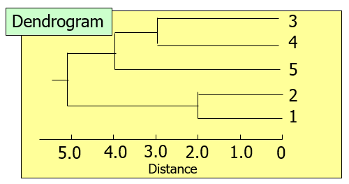
Hierarchic grouping can be represented by two-dimensional diagram known as dendrogram.

2.4a Agglomerative hierarchical clustering

Single Linkage

Also known as the nearest neighbor technique.

Distance between groups equals to the distance of the closest pair of data.

Complete Linkage

Distance between groups equals to the distance of the most distant pair of data.

Group Average Linkage

Distance between groups equals to the average of the distances between all pairs of records (one from each cluster).

Centroid Linkage

Distance between groups equals to the distance between the mean vectors of the two clusters.

Median Linkage

Disadvantage of the Centroid Clustering: When a large cluster is merged with a small one, the centroid of the combined cluster would be closed to the large one, ie. The characteristic properties of the small one are lost/

In median linkage, After we have combined two groups, the mid-point of the original two cluster centers is used as the new center of the newly combined group.

2.4B Divisive Methods

Polythetic Approach (Based on Group Average Linkage)

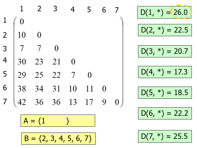
For the first iteration, calculate the distance between each point and the rest points. Choose the one with the largest distance to form the initial division.

Example:

In the following iterations:

• Calculate the distance between each point and A/B as $Dist_A$ and $Dist_B$
• Calculate the difference of $Dist_A$ and $Dist_B$ = $Dist_B - Dist_A$
• Choose the point with the largest distance difference and put it into A.

Example:

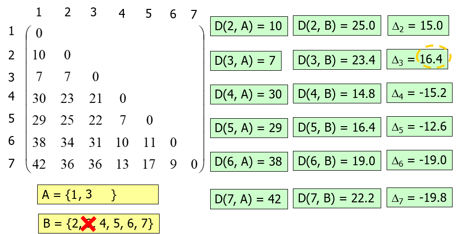
End the iteration when all differences are negative. The process would continue on each subgroup separately.

Monothetic Approach

It is usually used when the data consists of binary variables.

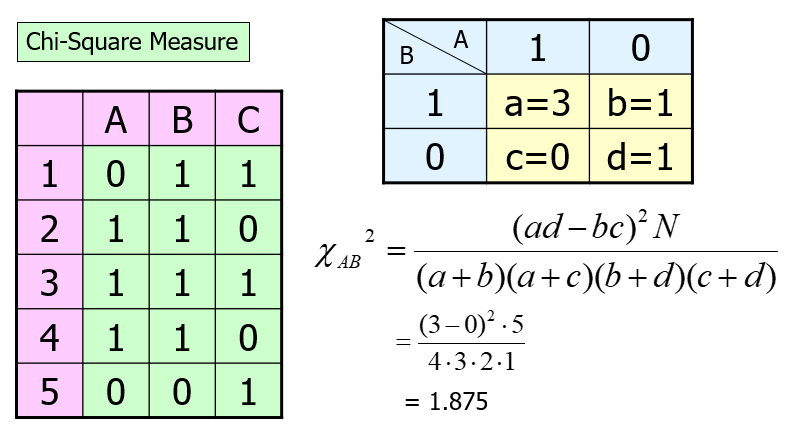
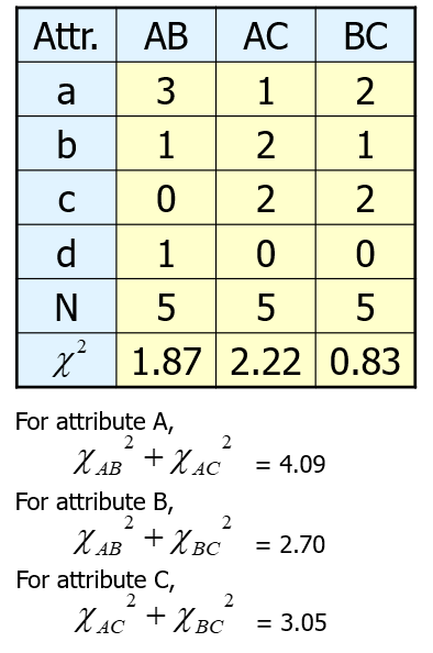
In this case, choose attribute A for dividing the data into two groups {2,3,4} and {1,5}

---

3 Classification

3.1 Decision Tree

ID3

Entropy is used to measure how informative is a node. When given a probability distribution $P = (p_1 , p_2 , ... , p_n)$, then the Information (or the Entropy of P) is:

$$I(P) = - p_1 log\ p_1 - p_2 log\ p_2 - ... - p_n log\ p_n$$

The Entropy is a way to measure the amount of information. The smaller the entropy is, the more information we have.

ID3 Impurity Measurement:

$$Gain(A,T) = Info(T)-Info(A,T)$$

C4.5

C4.5 Impurity Measurement:

$$Gain(A,T) = (Info(T) - Info(A,T))/SplitInfo(A)\\ where\ SplitInfo(A)=-\Sigma_{v\in A}\ p(v)log\ p(v)$$

CART

CART Impurity Measurement:

$$Gini:\ Info(P)=1-\Sigma _ j p_ j ^ 2$$

3.2 Naïve Bayesian Classifier

Bayes Rule:

$$P(A|B)=\frac{P(B|A)P(A)}{P(B)},\ where\ A,B\ are\ random\ variables$$

Independent Assumption:

• Each attribute are independent

$$P(X,Y,Z\ |\ A)=P(X|A)\times P(Y|A)\times P(Z|A)$$

Naïve Bayes

Naïve Bayes Classification is based on the independent assumption.

Race	Income	Child	Insurance
black	high	no	yes
white	high	yes	yes
white	low	yes	yes
white	low	yes	yes
black	low	no	no
black	low	no	no
black	low	no	no
white	low	no	no

Suppose we want to calculate: $P(Yes\ |\ Race=white,Income=high,child=no)$

$$P(Yes\ |\ Race=white,Income=high,child=no)\\ =\frac {P(Race=white,Income=high,child=no\ |\ Yes)P(Yes)} {P(Race=white,Income=high,child=no)}\\ =\frac {P(Race=white|Yes)P(Income=high|Yes)P(child=no|Yes)P(Yes)} {P(Race=white,Income=high,child=no)}\\ =\frac {0.09375\times 0.5} {P(Race=white,Income=high,child=no)}\\ =\frac {0.046875} {P(Race=white,Income=high,child=no)}$$

With the same method, calculate:

$$P(Yes\ |\ Race=white,Income=high,child=no)\\ =\frac {0} {P(Race=white,Income=high,child=no)}$$

Therefore, we predict the following new person will buy an insurance:

Race	Income	Child	Insurance
white	high	no	?

3.3 Bayesian Belief Network

Bayesian Belief Network do not have independent assumption. Some attributes are dependent on other attributes. For example:

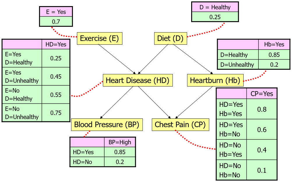
Conditionally independent

If $P(x\ |\ y,z) = P(x\ |\ z)$, x is conditionally independent of y given z. Also, if x is conditionally independent of y given z, $P(x,y\ |\ z)=P(x\ |\ z)\times P(y\ |\ z)$

In Bayesian Belief Network, a node is conditionally independent of its non-descendants if its parents are known.

Algorithm

Suppose there is a new person and we want to know whether he is likely to have Heart Disease:

Exercise	Diet	Heartburn	Blood Pressure	Chest Pain	Heart Disease
?	?	?	?	?	?

$$P(HD=Yes)\\ = \sum_{x\in\{yes,no\}} \sum_{y\in\{healthy,unhealthy\}} P(HD=Yes\ |\ E=x,D=y)\times P(E=x,D=y)\\ = \sum_{x\in\{yes,no\}} \sum_{y\in\{healthy,unhealthy\}} P(HD=Yes\ |\ E=x,D=y)\times P(E=x)\times P(D=y)\\ = 0.25\times0.7\times0.25+ 0.45\times0.7\times0.75+ 0.55\times0.3\times0.25+ 0.75\times0.3\times0.75 =0.49\\ P(HD=No)=1-P(HD=Yes)=1-0.49=0.51$$

---

Suppose there is a new person and we want to know whether he is likely to have Heart Disease:

Exercise	Diet	Heartburn	Blood Pressure	Chest Pain	Heart Disease
?	?	?	High	?	?

$$P(BP=High)=0.49\times0.85+0.51\times0.2=0.5185 \\ P(HD=Yes\ |\ BP=High)=\frac {P(BP=High\ |\ HD=Yes)P(HD=yes)} {P(BP=High)}\\ =\frac {0.85\times0.49} {0.5185}=0.8033\\ P(HD=No\ |\ BP=High)=1-P(HD=Yes\ |\ BP=High)=1-0.8033=0.1967$$

---

Suppose there is a new person and we want to know whether he is likely to have Heart Disease:

Exercise	Diet	Heartburn	Blood Pressure	Chest Pain	Heart Disease
Yes	Healthy	?	High	?	?

$$P(HD=Yes\ |\ E=Yes, D=Healthy, BP=High)\\ = \frac {P(BP=High\ |\ E=Yes, D=Healthy, HD=Yes)} {P(BP=High\ |\ E=Yes, D=Healthy)} \times P(HD=Yes\ |\ D=Healthy, E=Yes) \\ = \frac {P(BP=High\ |\ HD=Yes)\times P(HD=Yes\ |\ D=Healthy, E=Yes)} {\sum_{x\in\{yes,no\}}P(BP=High\ |\ HD=x)\times P(HD=x\ |\ E=Yes, D=Healthy)} \\ = \frac {0.85\times0.25} {0.85\times0.25+0.2\times0.75}=0.5862 \\ P(HD=No\ |\ E=Yes, D=Healthy, BP=High)\\ = 1- P(HD=Yes\ |\ E=Yes, D=Healthy, BP=High)\\ = 1-0.5862=0.4138$$

3.4 Nearest Neighbor Classifier

Algorithm

• Step 1: Find the nearest neighbor
• Step 2: Use the “label” of this neighbor

3.5 Support Vector Machine (SVM)

Advantages:

• Can be visualized.
• Accurate when data is well partitioned.

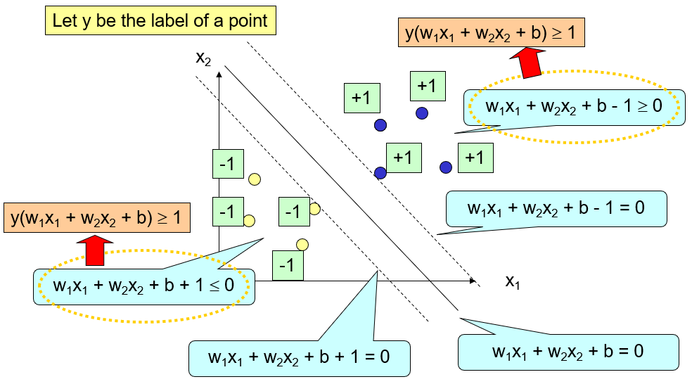
In this case: Margin equals to:

$$Margin = \frac {|(b+1)-(b-1)|} {\sqrt{\omega_1^2+\omega_2^2}} = \frac {2} {\sqrt{\omega_1^2+\omega_2^2}}$$

Therefore, maximize margin equals to minimize $\omega_1^2+\omega_2^2$, subject to $y(\omega_1x_1+\omega_2x_2+b)≥1$. where $y$ is the label of the point $(+1/-1).$

In this circumstance, we just described a 2-dimensional space. The space can be divided into two parts by a line.

For n-dimensional space where n ≥ 2. We use a hyperplane to divide the space into two parts.

Non-Linear Support Vector Machine:

• Step 1: Transform the data into a higher dimensional space using a “nonlinear” mapping.
• Step 2: Use the Linear Support Vector Machine in this high-dimensional space.

---

4 Neural Network

Neural Network is a computing system made up of simple and highly interconnected processing elements.

Information processing occurs at many identical and simple processing elements called neurons (or also called units, cells or nodes). Interneuron connection strengths known as synaptic weights are used to store the knowledge.

Advantage or Neural Network

• Parallel Processing.
• Fault Tolerance.

4.1 Activation Function

Threshold function

$$y= \begin{cases} 1,\ \ \ \ \ if\ x\geq0\\ 0,\ \ \ \ \ if\ x<0 \end{cases}$$

Linear function

$$y=x$$

Rectified Linear Unit (ReLU)

$$y= \begin{cases} x,\ \ \ \ \ if\ x\geq0\\ 0,\ \ \ \ \ if\ x<0\\ \end{cases}$$

Sigmoid

$$y= \frac {1} {1+e^{-net}}$$

tanh function

$$y= \frac {e^{2x}-1} {e^{2x}+1}$$

4.2 Learning

Let $\alpha$ be the learning rate.

Learning is done by:

• $\omega_i=\omega_i+\alpha(d-y)x_i$
• where $d$ is the desired output, $y$ is the output of the neural network
• $b = b+\alpha (d-y)$

When we processed all data points in the whole dataset, we say that we processed the dataset in one epoch. Data can be processed for multiple epochs.

Stopping condition:

The stopping condition could be specified with the following:

• The no. of epochs is equal to a specified number.

4.3 Multi-Layer Perception (MLP)

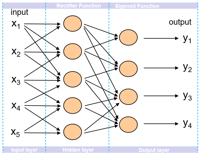
MLP can solve linear separable problems as well as non-linear separable problems.

MLP has proven to be a universal approximator. It can model all types function $y=f(x)$.

If the total number of layers is very large, this neural network is called a “deep network”. The processing of training a deep network and perform prediction with it is called “deep learning”.

Forward Propagation:

Based on the input and the current values of weight and bias variables, compute output $y$.

Backward Propagation

Based on the output $y$ and the desired output $d$, compute the error and update the variables.

---

5 Recurrent Neutral Network (RNN)

In neural network, we assume that records in the table are “independent”. In some cases, the current record is related to the previous records in the table. Thus, records in the table are “dependent”, we also want to capture this “dependency” in the model.

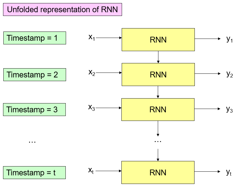
Limitation of RNN

• It may “memorize” a lot of past events.
• Due to its complex structure, it is more time-consuming for training.

5.1 Basic RNN

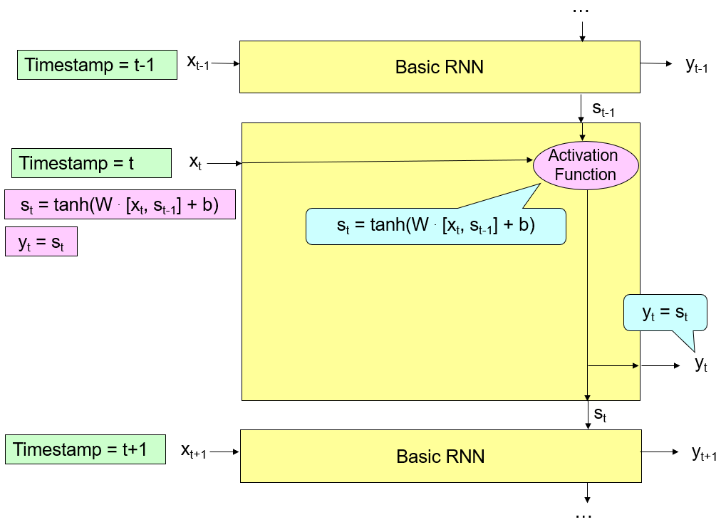
The Activation function of basic RNN is usually “tanh” or “ReLU”.

Similar to the neural network, the basic RNN model has two steps:

• Input Forward Propagation.
• Error Backward Propagation.

In the following, we focus on “Input Forward Propagation”. For RNN, “Error Backward Propagation” could be solved by an existing optimization tool.

5.2 LSTM (Long SHORT-term memory)

The basic RNN model is too “simple”. It could not easy for the basic RNN model to converge.

LSTM can simulate the brain process:

Forget Feature : It can forget a portion of the internal state variable.

Input Feature : It could decide to input a portion of the input variable for the model; It could decide the strength of the input for the model.

Output Feature : It could decide to output a portion of the output for the model; It could decide the strength of the output for the model.

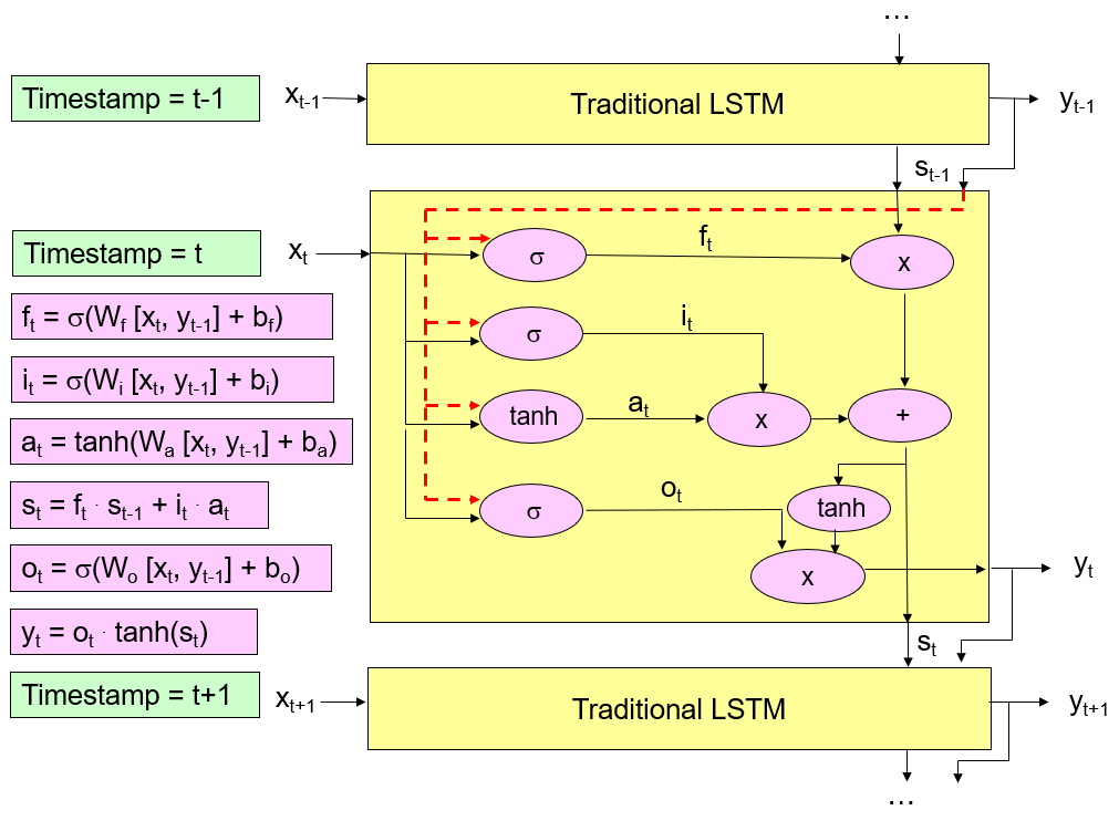
Similar to the “neural network”, the LSTM model could also have multiple layers and have multiple memory units in each layer.

5.3 GRU (Gated Recurrent Unit)

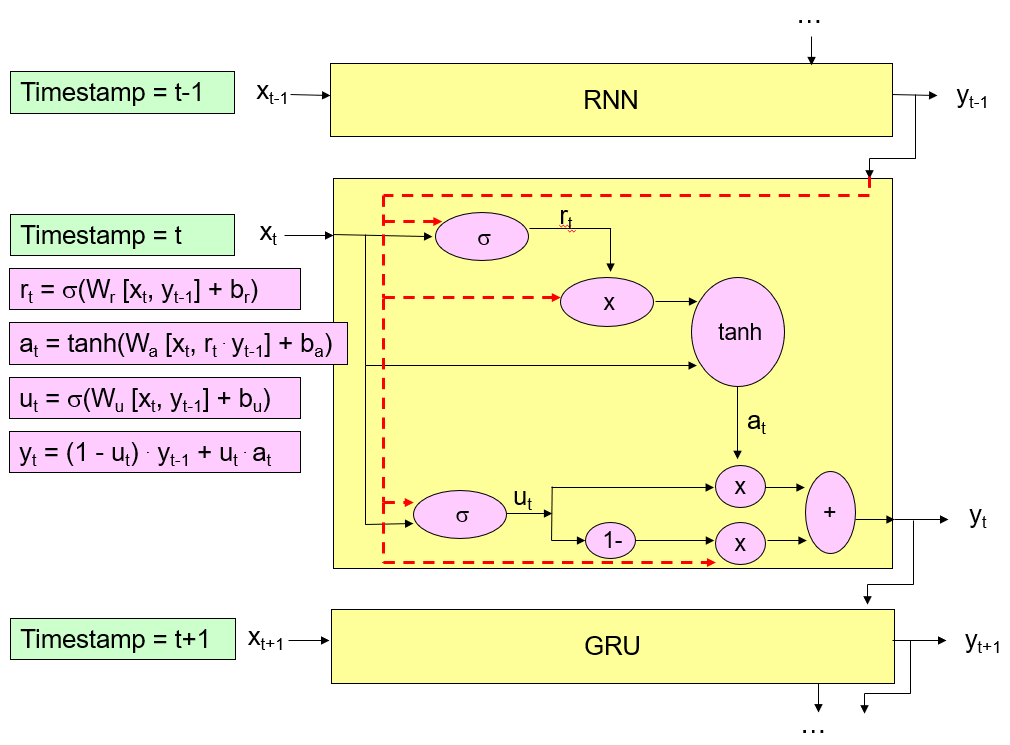
GRU is a variation of the traditional LSTM model. Its structure is similar to the traditional LSTM model, but its structure is “simpler”.

Advantage of GRU compared to traditional LSTM:

• The training time is shorter.
• It requires fewer data points to capture the properties of the data.

GRU model does not have an internal state variable to store our memory. It regards the “predicted” target attribute value of the previous record as a reference to store our memory.

Reset Feature : It could regard the “predicted” target attribute value of the previous record as a reference to store the memory.

Input Feature : It could decide the strength of the input for the model.

Output Feature : It could combine a portion of the predicted target attribute value of the previous record and a portion of the “processed” input variable.

---

6 Data Warehousing

Data warehousing is also called Online Analytical Processing (OLA)

Views structure:

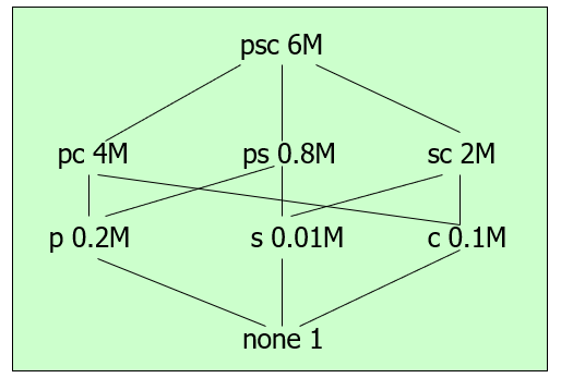
Selective Materialization Decision Problem is NP-hard

Algorithm (Greedy):

• S = {top view}
• For i = 1 to k do:
  • Select that view v not in S such that the benefit of selecting v is maximized.
  • Append S with v
• Resulting S is the greedy selection

---

7 Web Databases

7.1 HITS Algorithm

HITS is a ranking algorithm which ranks “hubs” and “authorities”.

$$a(v)=\Sigma_{u\to v} h(u)\\ h(v)=\Sigma_{v\to u} a(u)$$

HITS involves two major steps:

• Step1: Sampling Step
• Step2: Iteration Step

Sampling Step:

Collect a set of pages that are very relevant – called the base set.

Iteration Step

$$h=Ma\\ a=M^Th\\ Therefore,\ h=MM^Th,\ a=M^TMa$$

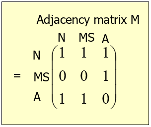
Rank Method:

• Rank in descending order of hub only
• Rank in descending order of authority only
• Rank in descending order of the value computed from both hub and authority

7.2 PageRank Algorithm (Google)

PageRank Algorithm makes use of Stochastic approach to rank the pages.